Part 2 – Tracking Motion

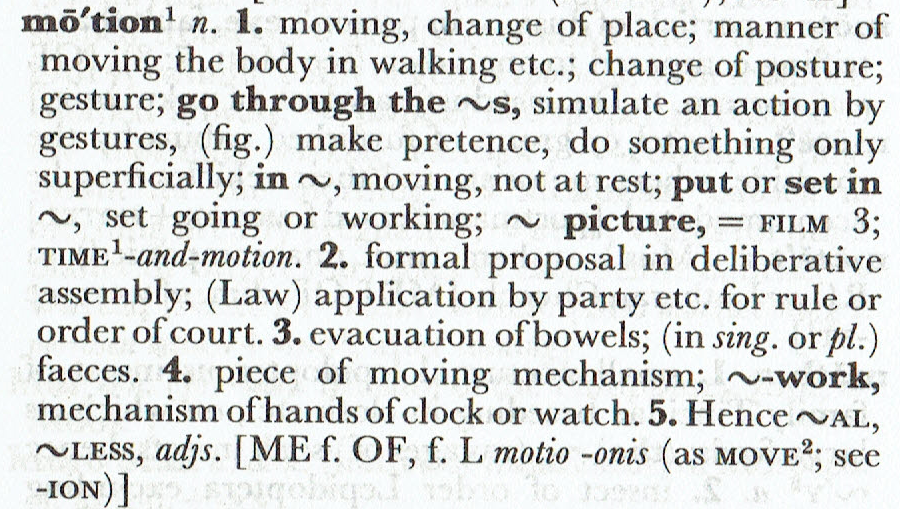
While I was thinking about which way to research this approach, it set me thinking about what motion was, or more specifically, what is a computer’s idea of motion.

Definition of Motion taken from OED

The answer would be that it would not understand motion, it would detect that the information contained within an image may have changed in comparison to the next one in a sequence but all we are talking about are specific 2D or 3D values associated with individual pixels within a specific colour space.

So to achieve a result that we would recognise as motion the computer has to take the pixel values and analyse the change in values in a way that we can use for tracking movement.

Centroid (find the centre of a blob)

So what is a blob exactly? in image processing terminology a blob is apparently a group of connected pixels sharing common values, and the centroid in this instance is the mean or average of this blob or the weighted average if you will.

OpenCV finds this weighted average with what is known as ‘moments’ by converting the image to grayscale, then perform binarisation before conducting the centroid calculations.

Multiple blobs can can be detected using this method within OpenCV with the aid of ‘contours’.

Meanshift & Camshift

Meanshift and Camshift can be used in conjunction with Centroid for the purposes of locating the part of the image we need to track.

Meanshift is a non-parametric density gradient estimation. It is useful for detecting the modes of this density. Camshift combines Meanshift with an adaptive region sizing step.

Both Meanshift and Camshift use a method called histogram back projection which uses colour as hue from a HSV model.

Results of my Camshift experiment on our allocated images.

Code for my Camshift program:

import sys
import numpy as np
import cv2
from matplotlib import pyplot as plt
import easygui

# Code written by Gavin Morrison D12124782

# Opening an image using a File Open dialog:
# f = easygui.fileopenbox()
# I = cv2.imread(f)

# Import image to be treated
original_image = cv2.imread("Ilovecat1.bmp")
	
# Copy of image to isolate region of interest
tracking_image = cv2.imread("Ilovecats1Copy.bmp")

# Coordinates of region of interest [row:row, column:column]
region_of_interest = tracking_image[125: 160, 210: 250]
	
	# Coordinates for right eye
	# region_of_interest = tracking_image[125: 175, 145: 200]
	
# The region of interest is converted to HSV colour space
HSV_region_of_interest = cv2.cvtColor(region_of_interest, cv2.COLOR_BGR2HSV)
	
#Create histogram of region of interest, using hue. The hue  range is from 0 to 179.
region_of_interest_histogram = cv2.calcHist([HSV_region_of_interest], [0], None, [180], [0, 180])

#Original image is converted to HSV colour space
original_image_HSV = cv2.cvtColor(original_image, cv2.COLOR_BGR2HSV)

# Back projection used to create mask from the hue of the region of interest histogram
mask = cv2.calcBackProject([original_image_HSV], [0], region_of_interest_histogram, [0, 180], 1)

# Filter applied in an attempt to reduce noise in the mask (later addition)
filter_kernel = cv2.getStructuringElement(cv2.MORPH_ELLIPSE, (3, 3))
mask = cv2.filter2D(mask, -1, filter_kernel)
_, mask = cv2.threshold(mask, 10, 255, cv2.THRESH_BINARY)
 
# The coordinates of our region of interest are assigned to variables
row = 210
column = 125
width = 250 - row
height = 160 - column
	
	# Coordinates for right eye
	# row = 145
	# column = 125
	# width = 200 - row
	# height = 175 - column

# define criteria
criteria = (cv2.TERM_CRITERIA_EPS | cv2.TERM_CRITERIA_COUNT, 10,1)

# rectangle of tracking area is created using camshift function 
rectangle, tracking_area = cv2.CamShift(mask, (row, column, width, height), criteria)

#These are the points for the rectangle
points = cv2.boxPoints(rectangle)
points = np.int0(points)
		
# cv2.polylines used instead of 'cv2.rectangle' to accommodate rotation of bound space. 
cv2.polylines(original_image, [points], True, (0, 255, 0), 2)

# Display our processed image
finished_image = cv2.cvtColor(original_image, cv2.COLOR_BGR2RGB)
plt.subplot(111),plt.imshow(finished_image,cmap = 'gray'), plt.title('Camshift Result'), plt.xticks([]), plt.yticks([])
plt.show()

import sys

import numpy as np

import cv2

from matplotlib import pyplot as plt

import easygui

# Code written by Gavin Morrison D12124782

# Opening an image using a File Open dialog:

# f = easygui.fileopenbox()

# I = cv2.imread(f)

# Import image to be treated

original_image = cv2.imread("Ilovecat1.bmp")

# Copy of image to isolate region of interest

tracking_image = cv2.imread("Ilovecats1Copy.bmp")

# Coordinates of region of interest [row:row, column:column]

region_of_interest = tracking_image[125: 160, 210: 250]

# Coordinates for right eye

# region_of_interest = tracking_image[125: 175, 145: 200]

# The region of interest is converted to HSV colour space

HSV_region_of_interest = cv2.cvtColor(region_of_interest, cv2.COLOR_BGR2HSV)

#Create histogram of region of interest, using hue. The hue range is from 0 to 179.

region_of_interest_histogram = cv2.calcHist([HSV_region_of_interest], [0], None, [180], [0, 180])

#Original image is converted to HSV colour space

original_image_HSV = cv2.cvtColor(original_image, cv2.COLOR_BGR2HSV)

# Back projection used to create mask from the hue of the region of interest histogram

mask = cv2.calcBackProject([original_image_HSV], [0], region_of_interest_histogram, [0, 180], 1)

# Filter applied in an attempt to reduce noise in the mask (later addition)

filter_kernel = cv2.getStructuringElement(cv2.MORPH_ELLIPSE, (3, 3))

mask = cv2.filter2D(mask, -1, filter_kernel)

_, mask = cv2.threshold(mask, 10, 255, cv2.THRESH_BINARY)

# The coordinates of our region of interest are assigned to variables

row = 210

column = 125

width = 250 - row

height = 160 - column

# Coordinates for right eye

# row = 145

# column = 125

# width = 200 - row

# height = 175 - column

# define criteria

criteria = (cv2.TERM_CRITERIA_EPS | cv2.TERM_CRITERIA_COUNT, 10,1)

# rectangle of tracking area is created using camshift function

rectangle, tracking_area = cv2.CamShift(mask, (row, column, width, height), criteria)

#These are the points for the rectangle

points = cv2.boxPoints(rectangle)

points = np.int0(points)

# cv2.polylines used instead of 'cv2.rectangle' to accommodate rotation of bound space.

cv2.polylines(original_image, [points], True, (0, 255, 0), 2)

# Display our processed image

finished_image = cv2.cvtColor(original_image, cv2.COLOR_BGR2RGB)

plt.subplot(111),plt.imshow(finished_image,cmap = 'gray'), plt.title('Camshift Result'), plt.xticks([]), plt.yticks([])

plt.show()

REFERENCES:

Find the Center of a Blob (Centroid) using OpenCV (C++/Python) (accessed 2nd November 2018)
https://www.learnopencv.com

Meanshift and Camshift (accessed 02.11.2018)
https://docs.opencv.org/3.4.3/db/df8/tutorial_py_meanshift.html

Mean Shift Tracking (accessed 02.11.2018)
https://www.bogotobogo.com/python/OpenCV_Python/python_opencv3_mean_shift_tracking_segmentation.php

Back Projection (accessed 02.11.2018)
https://docs.opencv.org/2.4/doc/tutorials/imgproc/histograms/back_projection/back_projection.html

Bradski GR. Computer Vision Face Tracking For Use in a Perceptual User Interface. Microcomputer Research Lab, Santa Clara, CA, Intel Corporation.
http://citeseerx.ist.psu.edu/viewdoc/download;jsessionid=B9A5277FF173D0455494A756940F7E6B?doi=10.1.1.14.7673&rep=rep1&type=pdf

Gavin Morrison's Image Processing Blog

Personal Blog for the Image Processing Module of DT211C-4

Research & Implementation – Tracking Texture & Tracking Motion

Part 2 – Tracking Motion